Homography: The main idea behind many CV applications
Introduction
In this blog post I will try to explain to you what a homography matrix is and how it is calculated. There are a lot of applications that use homography like.
- Panorama and PhotoSphere mode in the camera app.
- Satellite maps.
- Augmented Reality(AR) Devices.
- Navigating in indoor environments or without GPS.
- Image/Video Stabilization.
Homography
Homography matrix is a 3x3 matrix that represents the transformation of points in an image plane to another image plane. Basically it maps the points in image B to points in image A.
\[\begin{bmatrix} x' \\ y' \\ 1 \\\end{bmatrix} = H \begin{bmatrix} x \\ y \\ 1 \\ \end{bmatrix}\]\(x’, y’\) represents the points of imageB(\(x, y\)) in imageA plane.
Homography works well when the camera motion is restricted to only rotation and there is no translation motion. To explain why this is the case let’s look at the following visualization.
If we translate the camera we sometimes get into a situation where a few points line up as you can see in the visualization above(Refresh for new points). This causes the overlapping region of the image to look different in both the images. Stitching such images together will create artefacts in the resulting output.
However if what you are imaging lies in a plane the above problem does not occur as the points in the image cannot line up as you can see with the visualization below.
This is the case in satellite images. Those images are taken from such a great height that you can assume that all the points lie on the ground plane.
Feel free to play with the interactive visualisations to get a deeper intuition. Refresh the page to get different points.
Calculating Homography
Now let’s try to understand how to find the homography matrix given two images.
The process can be divided into 4 parts.
- Feature Detection
- Feature Description
- Feature Matching
- Calculating Homography Using RANSAC
Feature Detection
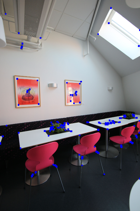
First part is to detect features in the images that we can use to compare the two images. Good features are generally those that can be localized in an image easily like corners, edges, blobs of color on a flat background etc.

Feature Description
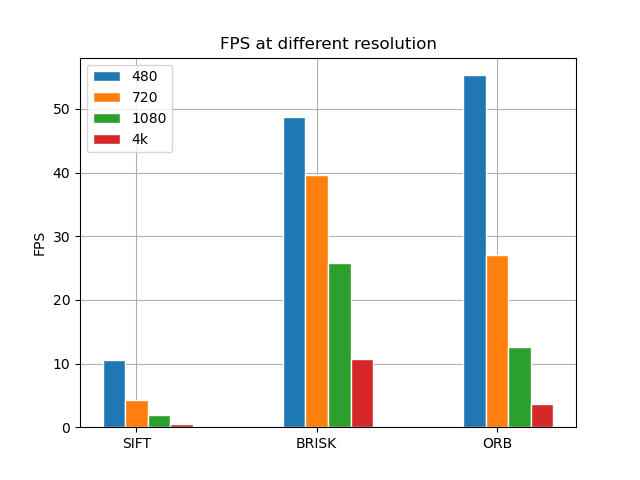
Now we want to describe the above features in a way so that we can compare them across images. A good description should be invariant to intensity, perspective change and should be fast to compute, compare and store. Some standard descriptors are - SIFT, BRISK and ORB. This is a great place to learn about them.
Here is a speed comparison of different descriptors for different resolutions on my system.

Feature Matching
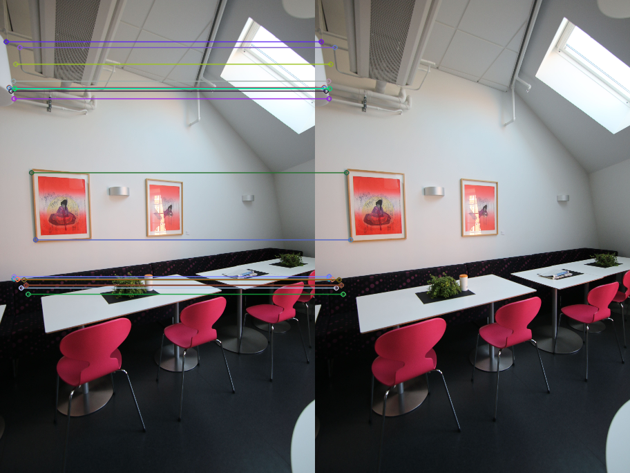
Now that we have the features and their descriptors we will use a matching algorithm to match these features together between different images. This will give us a pair of points that are the same in both the images which we can use to compute the Homography matrix in the next step. This can be done by comparing the distance between the feature descriptors that we calculated above of both the images.

RANSAC
In this step we use the RANSAC algorithm to find the homography matrix. The homography matrix has 8 unknown variables and so we need minimum 4 point matches to calculate the homography matrix. We generally use RANSAC which is an iterative method that tries different hypotheses and chooses the hypothesis that is most consistent with the data. This helps us deal with bad matches(outliers). You can read more here.
Here is the function for calculating the Homography in python using OpenCV.
feature_detector = cv2.SIFT_create()
matcher = cv2.BFMatcher()
def homography(image_a, image_b, feature_detector, matcher):
    # Detect features and compute there descriptors.
    kp_a, des_a = feature_detector.detectAndCompute(image_a, None)
    kp_b, des_b = feature_detector.detectAndCompute(image_b, None)

    # Match keypoints between those images.
    matches = matcher.knnMatch(des_a, trainDescriptors=des_b, k=2)
    # Discard bad matches.
    good_matches = []
    for m, n in matches:
        if m.distance < .75 * n.distance:
            good_matches.append(m)

    src_pts = np.float32([kp_a[m.queryIdx].pt for m in good_matches]).reshape(-1, 1, 2)
    dst_pts = np.float32([kp_b[m.trainIdx].pt for m in good_matches]).reshape(-1, 1, 2)

    # Compute the homography matrix if there are more than 4 matched points else return a zero matrix.
    if len(src_pts) > 4:
        M, mask = cv2.findHomography(dst_pts, src_pts, cv2.RANSAC, 5)
    else:
        M = np.array([[0, 0, 0], [0, 0, 0], [0, 0, 0]])
    return M
Conclusion
In this blog post I tried to summarise my understanding of the Homography matrix. In the next post I will try to use this knowledge to build some useful application.
I would love to hear your ideas and feedback in the comments below.
Useful Links
A great blog post on image stitching